ComfyUI-RK-Sampler

Batched Runge-Kutta Samplers for ComfyUI

Supports most practical Explicit Runge-Kutta (ERK) methods.

Tested on SD1.5, SDXL, and SD3.

Features

• Parallel ODE solvers for fast batch processing
• Explicit and Embedded Explicit Runge-Kutta methods
• PID controller for adaptive step sizing with tunable settings
• Scheduled controller for fixed step sizing (determined by the given $\sigma$ schedule)

Installation

ComfyUI-Manager

ComfyUI Manager Menu > Custom Nodes Manager > ComfyUI-RK-Sampler > Install

Manual installation

From ComfyUI/custom_nodes and ComfyUI virtual environment:

git clone https://github.com/wootwootwootwoot/ComfyUI-RK-Sampler.git
pip install torchode

Usage

Basic workflow

From Add Node:

sampling > custom_sampling > samplers > Runge-Kutta Sampler

Best defaults

• These methods support normal as well as high CFG scales, but the results may depend on the specific model.
• For SDXL, the best results I got were from CFG scales between 7-35.
• If you don't know the right step count or CFG scale:
  • Try the adaptive_pid controller with the base CFG and increment it until the results get worse.
  • Tune the CFG to the desired output.
  • Try the fixed_scheduled controller:
    • Use the Align Your Steps scheduler.
    • Set the scheduler's step count to be the same as the number of steps taken by the adaptive_pid controller.
    • Leave the CFG scale unchanged.
  • Tune the scheduler step count.
• When using adaptive_pid or adaptive_scipy controllers:
  • Set log_absolute_tolerance to -3.5:
    • Decrease it to set more strict tolerances (better results) in exchange for slower inference times.
    • Increase it to set less strict tolerances (worse results) in exchange for faster inference times.
  • Set log_relative_tolerance to be 1-2 more than log_absolute_tolerance.

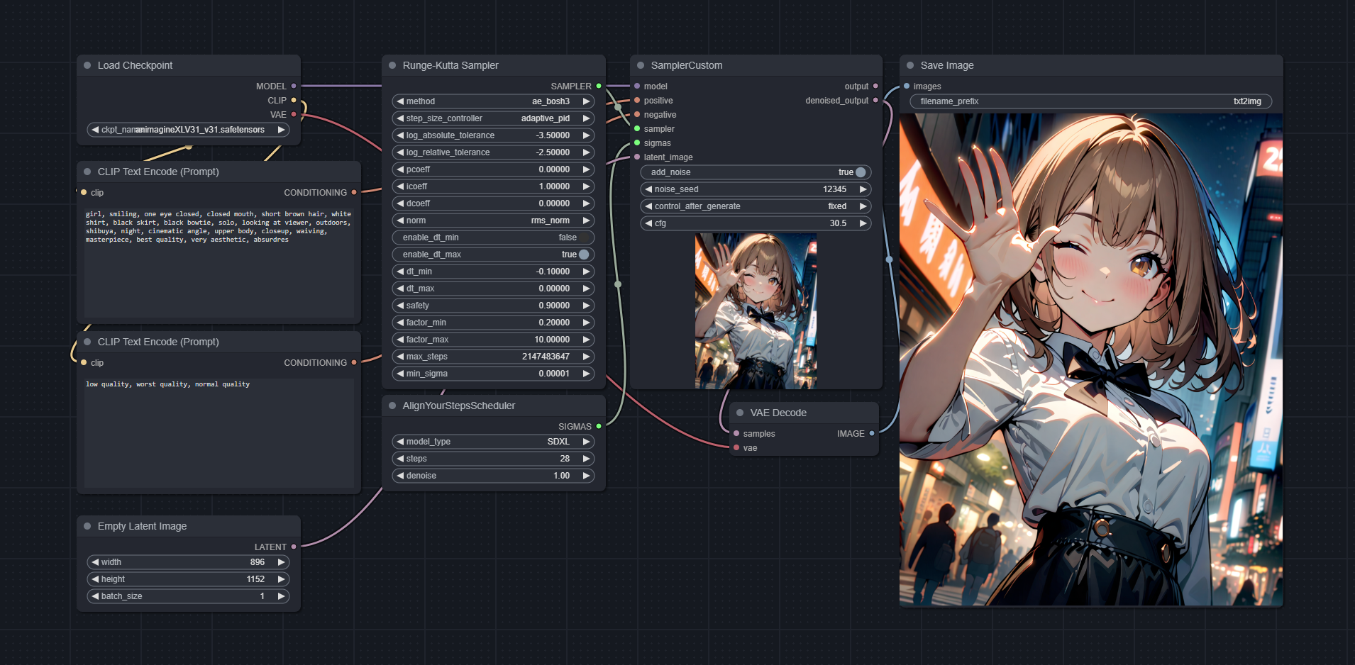
Adaptive step size

method: ae_bosh3
step_size_controller: adaptive_pid
log_absolute_tolerance: -3.5
log_relative_tolerance: -2.5
pcoeff: 0
icoeff: 1
dcoeff: 0
norm: rms_norm
enable_dt_min: false
enable_dt_max: true
dt_min: -0.1
dt_max: 0
safety: 0.9
factor_min: 0.2
factor_max: 10
max_steps: 2147483647
min_sigma: 1e-5
cfg: 7-35

Fixed step size

method: fe_ralston3
step_size_controller: fixed_scheduled
scheduler: Align Your Steps
steps: 28-150
cfg: 7-35

Choose a step size controller

step_size_controller: Controller to determine the step size taken on each sampling step.

adaptive controllers: Automatically determines the step size(s). The scheduler choice and scheduler step count does not matter since they only use the start and end timesteps.

fixed controllers: Uses the step size(s) provided by the scheduler. Works like a normal non-adaptive sampler in this case.

• adaptive_pid: A proportional–integral–derivative (PID) controller. Works with a-class methods.
• fixed_scheduled: A controller that uses the $\sigma$ (timestep) schedule from the scheduler. Works with a-class and f-class methods.
• adaptive_scipy: A basic integral controller wrapped from scipy. Works with s-class methods.

Choose a method

method: Determines the solver method used.

a, f, and s classes

• a = adaptive, f = fixed, s = scipy, e = explicit
• Use a-class methods with either:
  • adaptive_pid for automatically determined step sizes/count.
  • fixed_scheduled for scheduler determined step sizes/count.
• Use f-class methods with fixed_scheduled.
• Use s-class methods with adaptive_scipy.

Recommended methods

• Try ae_bosh3, ae_dopri5, and ae_fehlberg5 with the adaptive_pid step size controller.
• Try fe_ralston3, ae_bosh3, and fe_ssprk3 with the fixed_scheduled step size controller.

Quality ranking

Tested on RTX3090, SDXL, 896x1152, CFG=30, batch size 1, fixed_scheduled, Align Your Steps, 28 steps. | Rank | Name | Method | Order | NFEs | Time | | ----------- | ----------- | ----------- | ----------- | ----------- | ----------- | | 1 | fe_ralston3 | Ralston | 3 | 3 | 23.08s | | 2 | ae_bosh3 | Bogacki–Shampine | 3 | 3 | 23.03s | | 3 | fe_ssprk3 | Strong Stability Preserving Runge-Kutta | 3 | 3 | 22.97s | | 4 | fe_kutta4 | Runge-Kutta | 4 | 4 | 29.87s | | 5 | fe_kutta_38th4 | Runge-Kutta (3/8-rule) | 4 | 4 | 30.10s | | 6 | ae_dopri5 | Dormand–Prince | 5 | 6 | 44.03s | | 7 | ae_fehlberg5 | Runge–Kutta–Fehlberg | 5 | 6 | 44.28s | | 8 | ae_heun_euler2 | Heun–Euler | 2 | 2 | 15.87s | | 9 | fe_kutta3 | Runge-Kutta | 3 | 3 | 22.83s | | 10 | ae_ralston2 | Ralston | 2 | 2 | 16.05s | | 11 | ae_cash_karp5 | Cash-Karp | 5 | 6 | 44.47s | | 12 | fe_ralston4 | Ralston | 4 | 4 | 29.69s | | 13 | fe_euler1 | Forward Euler | 1 | 1 | 9.00s | | 14 | fe_wray3 | van der Houwen and Wray | 3 | 3 | 22.96s | | 15 | fe_heun3 | Heun | 3 | 3 | 23.13s | | 16 | ae_tsit5 | Tsitouras | 5 | 6 | 43.90s | | 17 | ae_midpoint2 | Explicit midpoint | 2 | 2 | 15.97s | | 18 | ae_fehlberg2 | Runge–Kutta–Fehlberg | 2 | 3 | 23.23s | | 19 | ae_dopri8 | Dormand–Prince | 8 | 13 | 94.10s |

Explicit methods from scipy.integrate

These methods are wrapped implementations of explicit solvers from scipy.integrate. | Name | Method | Order | NFEs | | ----------- | ----------- | ----------- | ----------- | | se_RK23 | Runge-Kutta | 3 | 3 | | se_RK45 | Runge-Kutta | 5 | 6 | | se_DOP853 | Dormand-Prince | 8 | 12 |

Solver settings

| Option | Applies to | Description | | ----------- | ----------- | ----------- | | method | adaptive_pid, fixed_scheduled, adaptive_scipy | Solver method. | | step_size_controller | adaptive_pid, fixed_scheduled, adaptive_scipy | Step size controller. | | log_absolute_tolerance | adaptive_pid, adaptive_scipy | $log_{10}$ of the threshold below which the solver does not worry about the accuracy of the solution since it is effectively 0. log_absolute_tolerance must be less than or equal to log_relative_tolerance. | | log_relative_tolerance | adaptive_pid, adaptive_scipy | $log_{10}$ of the threshold for the relative error of a single step of the integrator. | | pcoeff | adaptive_pid | Coefficients for the proportional term of the PID controller. | | icoeff | adaptive_pid | Coefficients for the integral term of the PID controller. P/I/D of 0/1/0 corresponds to a basic integral controller. | | dcoeff | adaptive_pid | Coefficients for the derivative term of the PID controller. | | norm | adaptive_pid, adaptive_scipy | Normalization function for error control. Step sizes are chosen so that norm(error / (absolute_tolerance + relative_tolerance * y)) is approximately one. | | enable_dt_min | adaptive_pid, adaptive_scipy | Enable clamping of the minimum step size to take to dt_min. | | enable_dt_max | adaptive_pid, adaptive_scipy | Enable clamping of the maximum step size to take to dt_max. | | dt_min | adaptive_pid, adaptive_scipy | The dt_min value to clamp to. Since we are solving a reverse-time ODE, this value should be negative. dt_min must be less than or equal to dt_max. | | dt_max | adaptive_pid, adaptive_scipy | The dt_max value to clamp to. Since we are solving a reverse-time ODE, this value should be negative. Clamped to 0 by default to force a monotonic solve. | | safety | adaptive_pid, adaptive_scipy | Multiplicative safety factor. | | factor_min | adaptive_pid, adaptive_scipy | Minimum amount a step size can be decreased relative to the previous step. factor_min must be less than or equal to factor_max. | | factor_max | adaptive_pid, adaptive_scipy | Maximum amount a step size can be increased relative to the previous step. | | max_steps | adaptive_pid, adaptive_scipy | Maximum amount of steps an adaptive step size controller is allowed to take. Taking more steps than max_steps will return an error. | | min_sigma | adaptive_pid, adaptive_scipy | Lower bound for $\sigma$ to consider the IVP solve to be complete. |

Comparison

Related projects

This extension improves upon ComfyUI-ODE by adding support for parallel processing, more controllability, high-quality live previews, a PID controller, and support for more fixed and adaptive step size solvers.

Speed

Tested on RTX3090, SDXL, 896x1152, CFG=30, adaptive_pid 0/1/0, ae_bosh3 (ComfyUI-RK-Sampler) / bosh3 (ComfyUI-ODE), log_absolute_tolerance=-3.5, log_relative_tolerance=-2.5. | Batch size | ComfyUI-RK-Sampler | ComfyUI-ODE | | ----------- | ----------- | ----------- | | 1 | 1m2s | 1m6s | | 2 | 2m3s | 2m7s | | 4 | 4m4s | 4m27s | | 8 | 7m39s | 9m3s | | 16 | 15m29s | 17m22s | | 32 | 30m18s | 36m34s |

Explanation

From Wikipedia:

In numerical analysis, the Runge–Kutta methods are a family of implicit and explicit iterative methods, which include the Euler method, used in temporal discretization for the approximate solutions of simultaneous nonlinear equations. These methods were developed around 1900 by the German mathematicians Carl Runge and Wilhelm Kutta.

The Runge-Kutta methods are a family of methods used for solving approximate solutions of ODEs by iterative discretization (or, if in diffusion terms, by sampling).

Runge-Kutta methods generally have less discretization error than standard diffusion sampling methods, allowing for the use of high CFG scales (within practical limits) to create high-quality results without artifacts.

Conditions for new solvers and methods

• No implicit solvers:
  • Implicit solvers require root-finding.
  • This means a backward pass through the model has to be ran to compute the Jacobian.
  • The Jacobian is then used during LBFGS optimization.
  • This is also very costly in terms of compute and memory usage.
• No non-RK methods:
  • This would cut off linear multistep methods like Adams-Bashforth or Adams predictor-corrector.
  • From my testing, RK methods perform better, even for explicit RK vs. predictor-corrector linear multistep.
• No duplicate methods:
  • If two methods have different coefficients, they aren't duplicates.
  • SciPy methods have different coefficients and implementations.

Changelog

24/07/24

• Added solver settings for adaptive_scipy.
• Progress bar improvements:
  • Adaptive solvers now show the number of steps taken.
  • Accurate $\sigma$ info is now displayed.
• Bugfixes and small refactors.

23/07/24

• Installation from ComfyUI-Manager.
• Bugfixes and small refactors.

22/07/24

• Added wrappers for explicit solvers from scipy.integrate:
  • se_RK23
  • se_RK45
  • se_DOP853
• Some notes about the wrapped scipy solvers:
  • To use the new solvers, select adaptive_scipy as the step size controller.
  • No fixed step size controllers are available for wrapped scipy methods.
  • These methods do not support parallel IVP solve, meaning the batch elements are processed sequentially.
  • Implicit solvers from scipy.integrate were skipped as the root finding step takes too long.
• The refactors from this update can cause the results to differ from the previous version. This is due to changes in floating point precision casting and operation orders.